Demystifying Tensor Parallelism

Modes of parallelism

Tensor Parallel (aka Tensor Model Parallel or TP) is a deep learning execution strategy that splits a model over multiple devices to enable larger models and faster runtime. It is one of the 3D parallelisms, alongside Data Parallel and Pipeline Parallel, which can be combined. All these are execution strategies, which means when enabled, the model remains mathematically equivalent, as opposed to strategies like quantisation, distillation or Mixture of Experts, which are model architectural changes.

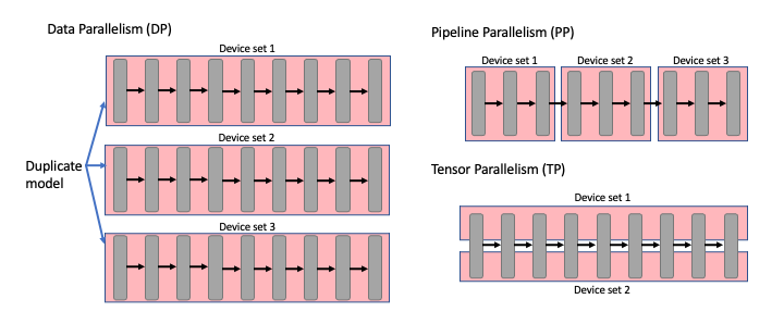Figure 1: A comparison of different modes of parallelism for a model made up of multiple sequential layers.

Data Parallelism is whereby each device has a replica of the model, the input batch is then split, and each replica processes a different sample. This allows the model to utilise more devices and increase throughput. However, there is a limit to how much you can split the batch; it reaches a point of indivisibility, and smaller data sizes may not effectively harness the available hardware. Also, the model must be able to fit in memory on a single device.

For Pipeline Parallelism, layers are assigned to different devices and processed as stages. This allows you to run models which would not otherwise fit into the memory of one device. The data is then sequentially processed by the device sets. Pipeline Parallelism inherently has warm-up and warm-down phases that only utilise some devices and decrease efficiency. Additionally, it’s essential to balance the load between stages; otherwise, devices will become underutilised (known as bubbles). This makes efficient implementations quite complex and requires a large batch size. The IPU Programming Guide has a good overview of the topic.

Tensor Parallelism is whereby a single layer is split across multiple devices, known as sharding. Care must be taken to ensure the output remains unchanged, and this is usually achieved by doing additional collective communication (All-Reduce, All-Gather, etc.) to sync the result between the devices. Suboptimal partitioning of the model can dramatically increase communication overheads, so using an efficient sharding scheme is essential. For instance, for some large models, communication can consume 50-70% of runtime. In the next section, we will discuss common sharding schemes.

Mode	Pros	Cons
Data Parallelism (DP)	Higher throughput Simple design Communication cost is small and only required for training	Batch size must be divisible by the number of DP nodes Model must fit into a single device set
Pipeline Parallelism (PP)	Increases memory capacity Small communication cost	Complex design Requires a large batch size Difficult to use in eager execution mode Pipeline warm-up, warm-down and bubbles decrease efficiency The number of layers must be divisible by the PP nodes
Tensor Parallelism (TP)	Higher throughput Increase memory capacity	Large communication cost The TP data axis must be divisible by the number of TP nodes

Data Parallelism and sometimes Tensor Parallelism result in tensors being replicated between devices. To save on memory, these replicated tensors can be sharded and collected between the devices when needed. This is known at Graphcore as Replicated Tensor Sharding, while DeepSpeed call it the ZeRO Redundancy Optimiser and PyTorch calls it Fully Sharded Data Parallel.

How to shard layers

Let’s start by looking at sharding a matrix multiplication (matmul) operation. Given an input $X$ with size $[n, m]$ and weights $A$ with size $[m, k]$, the operation is defined as:

\[\begin{gathered} f(X)=X A \\ X A=\left(\begin{array}{ll} X_{0} & X_{1} \\ X_{2} & X_{3} \end{array}\right)\left(\begin{array}{ll} A_{0} & A_{1} \\ A_{2} & A_{3} \end{array}\right) \\ X A=\left(\begin{array}{ll} X_{0} A_{0}+X_{1} A_{2} & X_{0} A_{1}+X_{1} A_{3} \\ X_{2} A_{0}+X_{3} A_{2} & X_{2} A_{1}+X_{3} A_{3} \end{array}\right) \end{gathered}\]

Above, you can consider $X$ and $A$ as 2 by 2 matrices or block matrices with 4 blocks each - both are equivalent.

A block matrix, also known as a partitioned matrix, is just a matrix of matrices. You can treat block matrices similarly to normal matrices. If A and B are block matrices whereby the blocks are partitioned appropriately, then matrix multiplication and addition remain unchanged. However, if you transpose a block matrix, you also need to transpose its elements (this becomes obvious if you consider the shapes of the blocks).

Next, we will have a look at common matmul sharding schemes. First, let’s consider whether to shard the weights column-wise or row-wise.

Column-wise sharding

Consider splitting the weights column-wise. The shape of each weight shard will be $[\mathrm{m}, \mathrm{k} / 2]$, as the first axis of $A$ is unchanged, we can provide the input $X$ with the same shape. We can assign each shard to a different device and duplicate $X$ across devices.

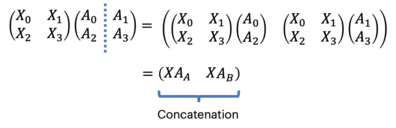
The operation output is also sharded column-wise across the devices. To realise the unsharded result on all devices, we need to concatenate the two shards. This can be done with an All-Gather, an MPI-style collective, which collects the sharded results and concatenates them to obtain the full unsharded result (XA) on all devices.

To emphasise the point once more, you start with $X$ on both devices, $A_{A}$ on devices 1 and $A_{B}$ on device 2 . You do $X A_{A}$ on device 1 and $X A_{B}$ on device 2. On both devices, you do an All-Gather, which outputs $X A$.

Row-wise sharding

Now, let’s consider splitting the weights matrix row-wise into two blocks with shapes $[\mathrm{m} / 2, \mathrm{k}]$. We must also split $\mathrm{X}$ column-wise to make the weight’s shape compatible with the input $\mathrm{X}$. $\mathrm{X}$ will have two blocks with shapes $[\mathrm{n}, \mathrm{m} / \mathrm{k}]$

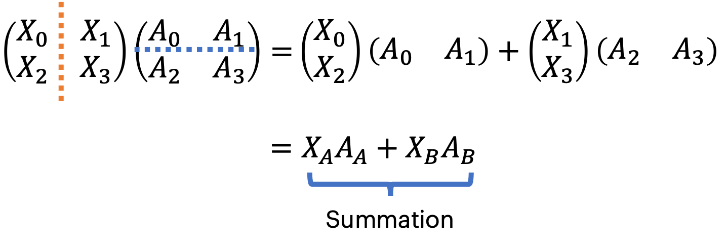
Notice how each device outputs a matrix of full size but with partial values. We need to sum up the two outputs to realise the unsharded result on all devices. This can be done with an All-Reduce, another MPI-style collective, which collects the results on all devices and sums them up.

Example: feed-forward transformer layer

Let’s apply the above to the feed-forward layer in a Transformer model, which is defined as (simplified version):

1. $X:=X A$
2. $X:=\operatorname{Gelu}(X)$
3. $Y:=X B$

In the above “layer” we have an input $X$ and produce output $Y$.

For each of the matrix multiplications (matmul), lines 1 and 3, we need to choose whether to shard them column or row-wise. The aim is to try to reduce the communication cost as much as possible, so it’s beneficial if we can “skip” a collective after a sharded matmul.

Let’s consider sharding the first matmul row-wise. Below is how it would work by representing the two devices as a tuple, and we have the input sharded on both devices $\left(X_{0}, X_{1}\right)$:

1. $\left(X_{0}, X_{1}\right):=\left(X_{0} A_{0}, X_{1} A_{1}\right)$
2. $(X, X):=\operatorname{AllReduce}(X_{0}, X_{1})$
3. $(X, X):=(\operatorname{Gelu}(X), \operatorname{Gelu}(X))$
4. $\left(X_{0}, X_{1}\right):=\left(X B_{0}, X B_{1}\right)$
5. $(Y, Y):=\operatorname{AllGather}(X_{0}, X_{1})$

The first matmul produces a partial output and requires an All-Reduce to realise the full result. The next is the activation function Gelu, which is an elementwise operation and non-linear. Because it’s non-linear, the Gelu would require the full result to produce the same numerical output, so we can’t skip the All-Reduce from the previous matmul - no luck here.

Next, we now try considering sharding the first matmul column-wise

1. $\left(X_{0}, X_{1}\right):=\left(X A_{0}, X A_{1}\right)$
2. $\left(X_{0}, X_{1}\right):=\left(\operatorname{Gelu}(X_{0}), \operatorname{Gelu}(X_{1})\right)$
3. $\left(X_{0}, X_{1}\right):=\left(X_{0} B_{0}, X_{1} B_{1}\right)$
4. $(Y, Y):= \operatorname{AllReduce}(X_{0}, X_{1})$

This produces a column-wise sharded output from the first matmul. Next, the Gelu is a pointwise operation that doesn’t require the full data to produce the same result. If we use row-wise sharding for the second matrix multiplication, the input must be shared column-wise, which matches up nicely with the previous result. This pattern of using column-wise followed by rowwise sharding is called pairwise sharding and reduces the number of collectives by half.

Pairwise sharding eliminates replicated compute on both devices and reduces inter-device communication. Pairwise sharding can also be applied to other layers, such as the Attention layer in a Transformer model

Gradients of tensor parallel layers

Determining how to calculate the gradient of a tensor parallel layer is non-trivial. This is because the autograd feature for most frameworks only considers a single device. First, a handwaving answer is provided on determining the gradients and then a full derivation.

Short answer

Column-wise or row-wise sharding

To determine how the gradient should be calculated, let’s consider the gradient of the input $X$ of a matrix multiplication layer with respect to the loss:

\[\begin{aligned} Y &= XA \\ \frac{\partial l}{\partial X} &= \frac{\partial l}{\partial Y} \frac{\partial Y}{\partial X}=\frac{\partial l}{\partial Y} A^{T} \end{aligned}\]

Notice how the weights $A$ are transposed when calculating the gradient, this means if the weights are row-wise sharded for the forward computation, they are column-wise sharded to calculate the gradient, and visa-versa. For simplicity, we shall call this process “flipping”.

Pairwise sharding

For pairwise sharding, let’s take the previous example of a feed-forward layer, defined as:

1. $X:=X A$
2. $X:=\operatorname{Gelu}(X)$
3. $Y:=X B$

In the above “layer” we have an input $X$, which we overwrite for each operation until we produce output $Y$

When doing backpropagation, you proceed through each layer backwards ( $B$ first and then $A$ ). We are provided with the gradient of the forward output $Y^{\prime}$ and need to calculate the gradient of the forward input $X^{\prime}$ :

1. $Y^{\prime}:=Y^{\prime} B^{T}$
2. $Y^{\prime}:=\operatorname{Gelu}^{\prime}(Y^{\prime})$
3. $X^{\prime}:=Y^{\prime} A^{T}$

As both B and A are “flipped”, and we proceed through the operations in reverse order, the backwards of a pairwise sharded layer is also pairwise sharded.

From the previous section, the forward pass of the pairwise sharded feed-forward layer is defined as:

1. $\left(X_{0}, X_{1}\right):=\left(X A_{0}, X A_{1}\right)$
2. $\left(X_{0}, X_{1}\right):=\left(\operatorname{Gelu}(X_{0}), \operatorname{Gelu}(X_{1})\right)$
3. $\left(X_{0}, X_{1}\right):=\left(X_{0} B_{0}, X_{1} B_{1}\right)$
4. $(Y, Y):=\operatorname{AllReduce}(X_{0}, X_{1})$

So the backward pass of the pairwise sharded feed-forward layer is:

1. $\left(Y_{0}^{\prime}, Y_{1}^{\prime}\right):=\left(Y^{\prime} B_{0}, Y^{\prime} B_{1}\right)$
2. $\left(Y_{0}^{\prime}, Y_{1}^{\prime}\right):=\left( \operatorname{Gelu}^{\prime}(Y_{0}^{\prime}), \operatorname{Gelu}^{\prime}(Y_{1}^{\prime})\right)$
3. $\left(Y_{0}^{\prime}, Y_{1}^{\prime}\right):=\left(Y_{0}^{\prime} A_{0}, Y_{1}^{\prime} A_{1}\right)$
4. $\left(X^{\prime}, X^{\prime}\right):=\operatorname{AllReduce}(Y_{0}^{\prime}, Y_{1}^{\prime})$

Long answer

This section is heavy on the theory - if you need a refresher on how to derive gradients in deep learning, have a look at my post: a brief tour of backpropagation and multi-variable calculus.

Column-wise sharding

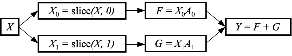
The computational graph for column-wise sharding is ($X$ and $A$ have the same shape and definitions as the previous section):

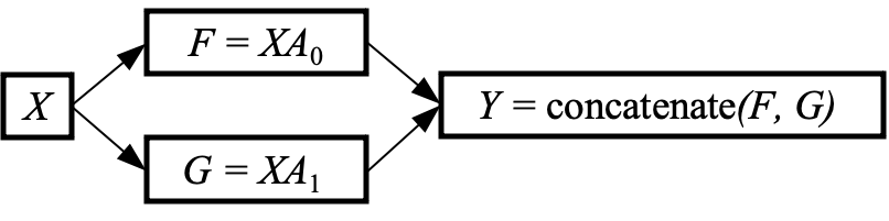
When performing backpropagation, we are provided the gradient of the loss / with respect to $Y$, and we need to calculate the gradient of the loss / with respect to $X$. We start with the multivariable chain rule as $Y$ is a function of both $F$ and $G$ :

\[\begin{aligned} \frac{\partial l}{\partial X} & =\frac{\partial l}{\partial Y}\left(\frac{\partial Y}{\partial F} \frac{\partial F}{\partial X}+\frac{\partial Y}{\partial G} \frac{\partial G}{\partial X}\right) \\ & =\operatorname{slice}\left(\frac{\partial l}{\partial Y}, 0\right) \frac{\partial F}{\partial X}+\operatorname{slice}\left(\frac{\partial l}{\partial Y}, 1\right) \frac{\partial G}{\partial X} \\ & =\operatorname{slice}\left(\frac{\partial l}{\partial Y}, 0\right) A_{0}^{T}+\operatorname{slice}\left(\frac{\partial l}{\partial Y}, 1\right) A_{1}^{T} \end{aligned}\]

First, the incoming gradient is split between the two paths due to the concatenation in the forward. In the final line, $A_{0}$ and $A_{1}$ are on different devices, so this summation can be performed using an All-Reduce. Notice how the all-reduce arises from the summation in the chain rule.

In summary, a column-wise sharded matmal is row-wise sharded in the backward computation.

Row-wise sharding

The computational graph for row-wise sharding is:

We first start by calculating the gradient of $Y$ with respect to $X$ using the multivariable chain rule:

1. $\frac{\partial Y}{\partial X}=\frac{\partial Y}{\partial F} \frac{\partial F}{\partial X_{0}} \frac{\partial X_{0}}{\partial X}+\frac{\partial Y}{\partial G} \frac{\partial G}{\partial X_{1}} \frac{\partial X_{1}}{\partial X}$
2. $\frac{\partial Y}{\partial X}=\frac{\partial F}{\partial X_{0}} \frac{\partial X_{0}}{\partial X}+\frac{\partial G}{\partial X_{1}} \frac{\partial X_{1}}{\partial X}$
3. $\frac{\partial Y}{\partial X}=A_{0}{ }^{T} \frac{\partial X_{0}}{\partial X}+A_{1}{ }^{T} \frac{\partial X_{1}}{\partial X}$
4. $\frac{\partial Y}{\partial X}=\operatorname{concatenate}\left(A_{0}{ }^{T}, A_{1}{ }^{T}\right)$

In line 3, $\partial X_{0} / \partial X$ is either 1 when the corresponding element of $X$ exists in $X_{0}$ or zero otherwise and similarly for $\partial X_{1} / \partial X . \partial X_{0} / \partial X$ and $\partial X_{1} / \partial X$ operate on mutually exclusive subsets of $X$, and therefore, we can combine them with a concatenation.

As $A_{0}$ and $A_{1}$ are located on different devices, an All-Gather can perform the concatenation.

When performing backpropagation, we are provided the gradient of the loss / with respect to $Y$, and we need to calculate the gradient of the loss / with respect to $X$ :

\[\begin{aligned} \frac{\partial l}{\partial X} & =\frac{\partial l}{\partial Y} \frac{\partial Y}{\partial X} \\ & =\frac{\partial l}{\partial Y} \text { concatenate }\left(A_{0}^{T},{A_{1}}^{T}\right) \end{aligned}\]

In summary, a row-wise sharded matmul is column-wise sharded in the backward computation.

Pairwise sharding

For pairwise sharding, the computational graph looks like this:

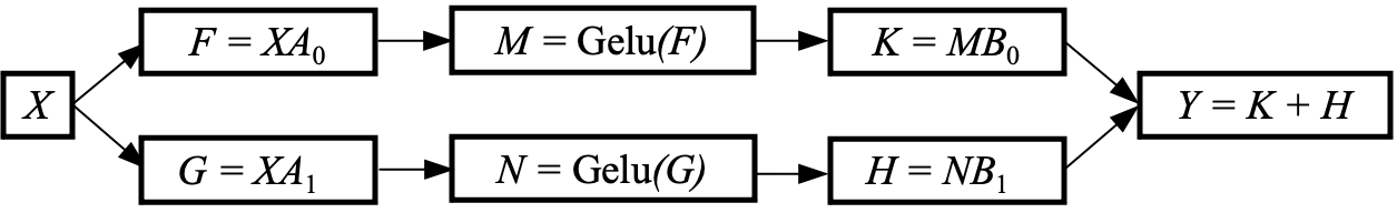
We first start by calculating the gradient of $Y$ with respect to $X$ using the multivariable chain rule:

\[\begin{aligned} \frac{\partial Y}{\partial X} &= \frac{\partial Y}{\partial K} \frac{\partial K}{\partial M} \frac{\partial M}{\partial F} \frac{\partial F}{\partial X}+\frac{\partial Y}{\partial H} \frac{\partial H}{\partial N} \frac{\partial N}{\partial G} \frac{\partial G}{\partial X} \\ &= B_{0}{ }^{T} \operatorname{Gelu}^{\prime}(F) A_{0}{ }^{T}+B_{1}{ }^{T} \operatorname{Gelu}^{\prime}(G) A_{1}{ }^{T} \end{aligned}\]

As the summands are located on different devices, an All-Reduce can perform the sum.

When performing backpropagation, we are provided the gradient of the loss / with respect to $Y$, and we need to calculate the gradient of the loss / with respect to $X$:

\[\begin{align*} \frac{\partial l}{\partial X} &= \frac{\partial l}{\partial Y}\frac{\partial Y}{\partial X} \\ &= \frac{\partial l}{\partial Y}\left ( {B_0}^T\textrm{Gelu}'(F){A_0}^T + {B_1}^T\textrm{Gelu}'(G){A_1}^T \right ) \end{align*}\]

In summary, pairwise sharding is pairwise sharded in the backward computation.

Implementation

There are currently three approaches to implementing tensor parallel.

SPMD (Single Program Multiple Data):

In the SPMD paradigm, a program is executed multiple times to run concurrently. Each instance of the program is allocated a set of resources (devices) and can operate across different machines. This method is facilitated by tools like PyTorch’s torchrun or the more general mpirun.

In practice, tensor parallelism is realised when each program instance manages different weight shards, and the user integrates necessary collective operations within the model script. This hands-on approach demands users to mathematically analyse their model’s operations to adapt it for tensor parallelism. Models such as Megatron or PopXL GPT-3 exemplify the use of this strategy.

Distributed Tensors

Distributed Tensors are whereby the framework provides the user with an interface that imitates normal tensors, hiding the fact that computing and storage are distributed. Tools such as PyTorch’s experimental DTensor or OneFlow implement this model. The primary benefit of this approach is its user-friendliness; it allows practitioners to leverage tensor parallel primitives without delving into the complexities of collective operation placement.

Automatic parallelism

As stated in the introduction, the most critical aspect of tensor parallelism is determining the optimal sharding strategy to minimise communication. Some recent efforts have been to provide automated tools such as Alpa; however, they have yet to be widely adopted or openly developed.

Summary

In the article, we discuss the three tensor parallel sharding schemes, which have different communication requirements:

• Column-wise sharding requires one All-Gather in the forward computation and one All-Reduce in the backward computation due to a column-wise sharded matmul being row-wise sharded in the backward computation.
• Row-wise sharding requires one All-Reduce in the forward computation and one All-Gather in the backward computation due to a row-wise sharded matmul being column-wise sharded in the backwards computation.
• Pairwise sharding requires one All-Reduce in the forward and one All-Reduce in the backward computation, due to a pairwise sharded layer is also pairwise sharded in the backward computation.